사람의 목소리의 높이는 음향적으로는 f0 값으로 나타낸다. 보통 청각적으로 느끼는 음의 높이를 염두에 두고 피치가 높다 낮다라고 표현하기도 한다.

 f0는 기본주파수(fundamental frequency)라고 부르기도 하는데 말하는 사람의 감정과 정서의 변화에 따라 달라진다.

 피치 값은 성대의 진동이 1초에 몇 번 있는가를 나타내는 것으로 성대의 크기와 길이, 질량 등에 영향을 받는다.

성대의 크기가 클수록 진동하는 속도가 느리기 때문에 여성보다 상대적으로 큰 성대를 가진 남성의 피치 값은 약 120 Hz가 된다.

 여성은 평균 약 230 Hz로 진동하며 어린아이는 300 Hz전후로 매우 높다.

 피치분석 알고리즘은 여러 가지가 나와 있으나 아직까지 소음이 섞인 음성이나 자음부분에 대한 측정상의 오류가 많이 나기 때문에 구한 값을 해석할 때 매우 주의해야 한다.

 특히, 성대 진동의 변화는 신체구조 상 서서히 변하는 데 비해, 음성분석은 지정한 크기의 창안에 있는 자료 앞뒤와는 별개로 분석하여 급작스럽게 변하는 오류 값을 나타내는 경우가 많기 때문에 주의해야한다.

PDA(Pitch detection algorithm)

Time domain과 Frequency domain 방식으로 나뉜다.

과제를 해나가면서, 제대로 하고 있는지 판단이 서지 않기 때문에 신뢰성 있는 프로그램과 비교해나가면서 하기로 했습니다.

해야할 작업을 나열하자면

1. 음성파형

2. 피치분석

3. 강도분석

4. 스펙트로그램 분석

5. 포먼트 분석 입니다.

1. 음성파형

Pratt 음성파형

Matlab 음성파형

2. 피치분석

Pratt 피치분석

3. 강도분석

Pratt 강도분석

MFCC를 하고있는데 왜 LPC를 하냐?

Matlab에서 포만트 관련 예제를 lpc로 하고있어서 입니다...

포만트에 대해서 간단히 언급한 후에 LPC를 통한 포만트 분석 후 이를 MFCC로 하겠습니다.

우선 소스

load mtlb;

segmentlen = 100;

noverlap = 90;

NFFT = 128;

[y,f,t,p] = spectrogram(mtlb,segmentlen,noverlap,NFFT,Fs);

surf(t,f,10*log10(abs(p)),'EdgeColor','none');

axis xy; axis tight; colormap(jet); view(0,90);

xlabel('Time');

ylabel('Frequency (Hz)');

dt = 1/Fs;

I0 = round(0.1/dt);

Iend = round(0.25/dt);

x = mtlb(I0:Iend);

x1 = x.*hamming(length(x));

preemph = [1 0.63];

x1 = filter(1,preemph,x1);

A = lpc(x1,8);

rts = roots(A);

rts = rts(imag(rts)>=0);

angz = atan2(imag(rts),real(rts));

[frqs,indices] = sort(angz.*(Fs/(2*pi)));

bw = -1/2*(Fs/(2*pi))*log(abs(rts(indices)));

nn = 1;

for kk = 1:length(frqs)

    if (frqs(kk) > 90 && bw(kk) <400)

        formants(nn) = frqs(kk);

        nn = nn+1;

    end

end

formants

------------------------------------------------------------

짧습니다. 실제 함수 하나하나 구현하려면 어렵겠지만요.

mtlb : 음원

segmentation : 분할... 이라는데. 해밍윈도우와 관련. 

noverlap : 앞서 MFCC에서의 overlap 부분.

NFFT : FFT resolution. 주파수 분해능, 

dt : 주기

IO와 len : 0.1~0.25초 때의 번호를 뜻합니다

x : mtlb의 0.1~0.25초 사이의 신호정보 입니다.

round는 가장 가까운 정수쪽으로 반올림을 합니다.

x1 : 해밍윈도우를 통과한 신호정보 입니다.

preemph : 프리엠퍼시스 필터의 적용입니다. 프리엠퍼시스 필터는 highpass all-pole(AR(1))필터라는데 all-pole이 무슨 뜻인지 모르겠네요. 이를 x1에 적용하였습니다.

필터관련은 나중에 더 공부하기로 하죠

A=lpc(x1,8) 을 통해서 신호 x1에 대하여 8개의  lpc ㄱ

앞서했던 STFT에 Mel_Frequency Filter Bank를 적용시키는 부분입니다.

Log Operation 까지 적용했습니다.

%% Adapt mel_filterbank

filter_demension=30;

MFB=melfilterbank(filter_demension, N, FS);

%Frequency to Mel-frequency

%주파수->멜주파수

Aspec=MFB*PSPEC;%Aspec:Audio Spectrogram

[mel_x,mel_y]=meshgrid(time,[1:filter_demension]);

figure;

mesh(mel_x,mel_y,Aspec);

%% Get Log Operation

LAspec=log(Aspec);

figure;

mesh(mel_x,mel_y,LAspec);

필터의 갯수를 30개로 하였습니다.

MFB는 멜 필터뱅크로 인수는 (필터갯수, NFFT(주파수 레졸루션, 2^9), FS(주파수 16000Hz))

Aspec는 오디오스펙트로그램으로 앞서 구한 MFB에 파워스펙트로그램인 PSPEC를 곱해줍니다.

AudioSpectrogram

LAspec는 로그를 적용한 오디오스펙트로그램입니다.

Loged AudioSpectrogram

앞서 spectrogram함수로 구한 스펙트로그램과 비슷하다는걸 알 수 있습니다. 정보의 용량이 대폭 줄었죠.

spectrogram

오늘 다루려고 하는것은 위의 melfilterbank(filter_demension, N, FS) 함수입니다.

사실 이 부분을 제대로 이해하지 못해서, 다른 matlab코드를 분석하면서 공부했죠...

함수 내용입니다.

-------------------------------------------------------------------------------

function m = melfilterbank(p, n, fs)

% The function computed the mel filter banks for robust speaker recognition

% The filter spectrum is such that the passband area remains the same yet

% the pasband frequencies decrease and the power increases, to emphasis the

% higher frequency components

% p number of filters in filterbank

% n length of fft

% fs sample rate in Hz

f0 = 700/fs;

fn2 = floor(n/2);                                   %16000/2=8000

lr = log(1 + 0.5/f0) / (p+1);                       %p+1만큼 등간격 등분

% convert to fft bin numbers with 0 for DC term

bl = n * (f0 * (exp([0 1 p p+1] * lr) - 1));

b1 = floor(bl(1)) + 1;

b2 = ceil(bl(2));

b3 = floor(bl(3));

b4 = min(fn2, ceil(bl(4))) - 1;

pf = log(1 + (b1:b4)/n/f0) / lr;

fp = floor(pf);

pm = pf - fp;

r = [fp(b2:b4) 1+fp(1:b3)];

c = [b2:b4 1:b3] + 1;

v = [1-pm(b2:b4) pm(1:b3)];

m= sparse(r,c, v, p, 1+fn2);

figure;

hold on

for num=1:p

    plot(m(num,:));

end

-------------------------------------------------------------------------------

사실 위 함수 말고도 다른 함수가 여럿 있었습니다만  이 함수가 제일 메모리를 적게 먹더군요.

그 이유가 바로 sparse함수 때문이었습니다.

매트릭스를 보면 0이 많은 경우가 많습니다. 사실 이런 데이터는 굳이 표현해 줄 필요가 없습니다.

예를들어 290*380의 매트릭스에서 60퍼센트 정도의 데이터가 0이면 이걸 다 표현해주면 290*380*0.6이라는 엄청난 메모리 낭비가 있습니다. 여기서 sparse를 이용해서 유효한 데이터의 값과 좌표데이터만 표현해 주자는 것이죠.

안드로이드 앱등의 플랫폼에 옮긴다고 할 때 메모리 문제는 굉장히 예민하게 다루어집니다. 이런 부분에서 세심한 배려가 제품의 가치를 높이는 것이겠죠.

그럼 함수 설명을 시작하겠습니다. 하나하나 짚어가면서 진행합니다.

일단 멜 필터뱅크 구축에 사용되는 함수는 두가지 입니다.

M(f)는 주파수를 Mel주파수로 바꿉니다.

M^(-1)(m)은 Mel주파수를 주파수로 바꿔줍니다.

여기서 주의, 1125라는 값을 보죠. M^(-1)(m)의 m에 M(f)를 대입시키면 1125/1125가 되어 f가 됩니다.

위 함수에서 1125값이 보이지 않는것은 이것 때문입니다.

음성 분석을 할 때, 주어지는 FS의 절반에 해당하는 주파수의 정보까지 얻을 수 있습니다.

FS=16000, 따라서 8000Hz까지 분석하게 되죠. 앞서 STFT에서 8000Hz까지 분석하는것도 같은 이유입니다.

lr 에서 /(p+1)을 제외하고 봅시다.

lr = log(1 + 0.5/f0);

f0 = 700/fs; 까지 대입시켜 보면

lr = log(1+0.5*fs/700) 으로 (1)식에서 1125를 제외한 식이 됩니다.

여기서 /(p+1)을 하는 이유는 (p+1)등분 하기 위해서이죠. 30개의 필터를 만든다고 하면 p+1=31로 나눕니다.

앞서 영문자료 보면 10개 필터를 만들경우 포인트를 +2한 12포인터를 잡습니다. 일단 이렇게 알아둡시다.

bl을 분석해 봅시다.

bl = n * (f0 * (exp([0 1 p p+1] * lr) - 1));

bl = n/FS * (700*(exp(m)-1))

exp([0 1 p p+1])의 0에서 31은 32의 길이를 갖습니다. 30+2이죠?

위 식은 n/FS를 제외하면 (2)식에 1125를 뺀것과 같습니다. 

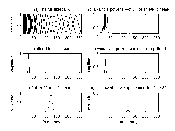
그럼 어째서 n/FS를 하느냐. 영문사이트 및 위에서 보는 그래프에 따르면 aplitude가 0~1로 표현되어 있습니다. 이와 같은 스케일로 표현하기 위해서 취해주었습니다.

실제로 bl의 결과가 0~256까지의 값이 나옵니다. 자연수로 해서 1단위로 보면 257의 길이를 갖습니다.

앞서 STFT에서 주파수 영역(0~8000)이 257개로 나뉜것과 같습니다.(STFT의 1+R/2=1+(2^9)/2과 같습니다.)

실제로 계산해보면 n*f/FS이기 때문에 (2^9)*(1/2)=256이 됩니다.

0 1 p p+1은 각각 용도가 있어서 넣은 값입니다.

b1 = floor(bl(1)) + 1;

b2 = ceil(bl(2));

b3 = floor(bl(3));

b4 = min(fn2, ceil(bl(4))) - 1;

bl(1)~bl(4)은 0 1 p p+1의 결과값입니다.

b1=1, b2=2, b3=234, b4=255가 됩니다.

----------------------------------------------------------------------여기까지 1단계로 봅시다.

pf를 식으로 표현하면 ln(1+ (b1:b4)*FS/(2^9)*1/700)/lr

pf가 가지는 값은 0에서 31 미만입니다.

fp는 버림을 적용함으로 0에서 30까지의 값을 가집니다.

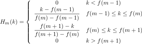
pm은 pf에서 정수부를 제거한 값입니다. 이것이 가지는 의의는 영문 자료의 아래의 식을 구현했다는 것입니다.

이는 0Hz에서 8000Hz까지를 257등분하여 0에서 256까지의 257단계의 자연수 스케일로 표시하고 각 필터(0에서 30)마다 0에서 257까지의 스케일에 대하여 갖는 결과값(Hm, 0에서 1사이)을 갖는다. 이는 3차원 공간에의 자료이다.

Matlab으로 영문자료와 같은 그래프를 출력하려고 할때 그냥 plot(데이터)를 해버리면

이런 결과가 나온다. 

실제 3차원으로 보는 필터는 다음과 같다.

X,Z평면으로 보면 다음과 같다.

2차원 plot으로 hold on과 for을 이용하여 출력하면 다음과 같다.

필터를 몇개 제거하여보자.

for i=0:3:30으로 필터를 10개정도 제거하여 보자

필터를 통과한 성분들만 남아있는 것을 알 수 있다.

Mel_FilterBank에 사용된 식이 어떻게 나왔는가, Matlab 코드에서 좌표와 소수점 이하 자료로 나누는 부분 등 다루고 싶은 부분이 많으나 아직 이해가 부족하고 시간이 많이 소모되므로 프로젝트가 끝난 후로 미루도록 하겠다.

Mel Frequency Cepstral Coefficient (MFCC) tutorial

The first step in any automatic speech recognition system is to extract features i.e. identify the components of the audio signal that are good for identifying the linguistic content and discarding all the other stuff which carries information like background noise, emotion etc.

The main point to understand about speech is that the sounds generated by a human are filtered by the shape of the vocal tract including tongue, teeth etc. This shape determines what sound comes out. If we can determine the shape accurately, this should give us an accurate representation of the phoneme being produced. The shape of the vocal tract manifests itself in the envelope of the short time power spectrum, and the job of MFCCs is to accurately represent this envelope. This page will provide a short tutorial on MFCCs.

Mel Frequency Cepstral Coefficents (MFCCs) are a feature widely used in automatic speech and speaker recognition. They were introduced by Davis and Mermelstein in the 1980's, and have been state-of-the-art ever since. Prior to the introduction of MFCCs, Linear Prediction Coefficients (LPCs) and Linear Prediction Cepstral Coefficients (LPCCs) and were the main feature type for automatic speech recognition (ASR). This page will go over the main aspects of MFCCs, why they make a good feature for ASR, and how to implement them.

Steps at a Glance 

We will give a high level intro to the implementation steps, then go in depth why we do the things we do. Towards the end we will go into a more detailed description of how to calculate MFCCs.

1. Frame the signal into short frames.
2. For each frame calculate the periodogram estimate of the power spectrum.
3. Apply the mel filterbank to the power spectra, sum the energy in each filter.
4. Take the logarithm of all filterbank energies.
5. Take the DCT of the log filterbank energies.
6. Keep DCT coefficients 2-13, discard the rest.

There are a few more things commonly done, sometimes the frame energy is appended to each feature vector. Delta and Delta-Delta features are usually also appended. Liftering is also commonly applied to the final features.

Why do we do these things? 

We will now go a little more slowly through the steps and explain why each of the steps is necessary.

An audio signal is constantly changing, so to simplify things we assume that on short time scales the audio signal doesn't change much (when we say it doesn't change, we mean statistically i.e. statistically stationary, obviously the samples are constantly changing on even short time scales). This is why we frame the signal into 20-40ms frames. If the frame is much shorter we don't have enough samples to get a reliable spectral estimate, if it is longer the signal changes too much throughout the frame.

The next step is to calculate the power spectrum of each frame. This is motivated by the human cochlea (an organ in the ear) which vibrates at different spots depending on the frequency of the incoming sounds. Depending on the location in the cochlea that vibrates (which wobbles small hairs), different nerves fire informing the brain that certain frequencies are present. Our periodogram estimate performs a similar job for us, identifying which frequencies are present in the frame.

The periodogram spectral estimate still contains a lot of information not required for Automatic Speech Recognition (ASR). In particular the cochlea can not discern the difference between two closely spaced frequencies. This effect becomes more pronounced as the frequencies increase. For this reason we take clumps of periodogram bins and sum them up to get an idea of how much energy exists in various frequency regions. This is performed by our Mel filterbank: the first filter is very narrow and gives an indication of how much energy exists near 0 Hertz. As the frequencies get higher our filters get wider as we become less concerned about variations. We are only interested in roughly how much energy occurs at each spot. The Mel scale tells us exactly how to space our filterbanks and how wide to make them. Seebelow for how to calculate the spacing.

Once we have the filterbank energies, we take the logarithm of them. This is also motivated by human hearing: we don't hear loudness on a linear scale. Generally to double the percieved volume of a sound we need to put 8 times as much energy into it. This means that large variations in energy may not sound all that different if the sound is loud to begin with. This compression operation makes our features match more closely what humans actually hear. Why the logarithm and not a cube root? The logarithm allows us to use cepstral mean subtraction, which is a channel normalisation technique.

The final step is to compute the DCT of the log filterbank energies. There are 2 main reasons this is performed. Because our filterbanks are all overlapping, the filterbank energies are quite correlated with each other. The DCT decorrelates the energies which means diagonal covariance matrices can be used to model the features in e.g. a HMM classifier. But notice that only 12 of the 26 DCT coefficients are kept. This is because the higher DCT coefficients represent fast changes in the filterbank energies and it turns out that these fast changes actually degrade ASR performance, so we get a small improvement by dropping them.

What is the Mel scale? 

The Mel scale relates perceived frequency, or pitch, of a pure tone to its actual measured frequency. Humans are much better at discerning small changes in pitch at low frequencies than they are at high frequencies. Incorporating this scale makes our features match more closely what humans hear.

The formula for converting from frequency to Mel scale is:

To go from Mels back to frequency:

Implementation steps 

We start with a speech signal, we'll assume sampled at 16kHz.

1. Frame the signal into 20-40 ms frames. 25ms is standard. This means the frame length for a 16kHz signal is 0.025*16000 = 400 samples. Frame step is usually something like 10ms (160 samples), which allows some overlap to the frames. The first 400 sample frame starts at sample 0, the next 400 sample frame starts at sample 160 etc. until the end of the speech file is reached. If the speech file does not divide into an even number of frames, pad it with zeros so that it does.

The next steps are applied to every single frame, one set of 12 MFCC coefficients is extracted for each frame. A short aside on notation: we call our time domain signal . Once it is framed we have where n ranges over 1-400 (if our frames are 400 samples) and  ranges over the number of frames. When we calculate the complex DFT, we get  - where the  denotes the frame number corresponding to the time-domain frame.  is then the power spectrum of frame .

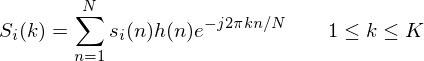
2. To take the Discrete Fourier Transform of the frame, perform the following:

where  is an  sample long analysis window (e.g. hamming window), and  is the length of the DFT. The periodogram-based power spectral estimate for the speech frame  is given by:

This is called the Periodogram estimate of the power spectrum. We take the absolute value of the complex fourier transform, and square the result. We would generally perform a 512 point FFT and keep only the first 257 coefficents.

3. Compute the Mel-spaced filterbank. This is a set of 20-40 (26 is standard) triangular filters that we apply to the periodogram power spectral estimate from step 2. Our filterbank comes in the form of 26 vectors of length 257 (assuming the FFT settings fom step 2). Each vector is mostly zeros, but is non-zero for a certain section of the spectrum. To calculate filterbank energies we multiply each filterbank with the power spectrum, then add up the coefficents. Once this is performed we are left with 26 numbers that give us an indication of how much energy was in each filterbank. For a detailed explanation of how to calculate the filterbanks see below. Here is a plot to hopefully clear things up:

4. Take the log of each of the 26 energies from step 3. This leaves us with 26 log filterbank energies.

5. Take the Discrete Cosine Transform (DCT) of the 26 log filterbank energies to give 26 cepstral coefficents. For ASR, only the lower 12-13 of the 26 coefficients are kept.

The resulting features (12 numbers for each frame) are called Mel Frequency Cepstral Coefficients.

Computing the Mel filterbank 

To get the filterbanks shown in figure 1(a) we first have to choose a lower and upper frequency. Good values are 300Hz for the lower and 8000Hz for the upper frequency. Of course if the speech is sampled at 8000Hz our upper frequency is limited to 4000Hz. Then follow these steps:

1. Using equation 1, convert the upper and lower frequencies to Mels. In our case 300Hz is 401.25 Mels and 8000Hz is 2834.99 Mels.
2. For this example we will do 10 filterbanks, for which we need 12 points. This means we need 10 additional points spaced linearly between 401.25 and 2834.99. This comes out to:

   m(i) = 401.25, 622.50, 843.75, 1065.00, 1286.25, 1507.50, 1728.74, 
          1949.99, 2171.24, 2392.49, 2613.74, 2834.99

3. Now use equation 2 to convert these back to Hertz:

   f(i) = 300, 517.33, 781.90, 1103.97, 1496.04, 1973.32, 2554.33, 
          3261.62, 4122.63, 5170.76, 6446.70, 8000

   Notice that our start- and end-points are at the frequencies we wanted.
4. Now we create our filterbanks. The first filterbank will start at the first point, reach its peak at the second point, then return to zero at the 3rd point. The second filterbank will start at the 2nd point, reach its max at the 3rd, then be zero at the 4th etc. A formula for calculating these is as follows:
   
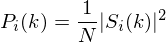
   where  is the number of filters we want, and  is the list of M+2 Mel-spaced frequencies.

The final plot of all 10 filters overlayed on each other is:

Deltas and Delta-Deltas 

Also known as differential and acceleration coefficients. The MFCC feature vector describes only the power spectral envelope of a single frame, but it seems like speech would also have information in the dynamics i.e. what are the trajectories of the MFCC coefficients over time. It turns out that calculating the MFCC trajectories and appending them to the original feature vector increases ASR performance by quite a bit (if we have 12 MFCC coefficients, we would also get 12 delta coefficients, which would combine to give a feature vector of length 24).

To calculate the delta coefficients, the following formula is used:

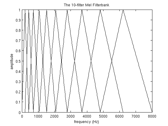
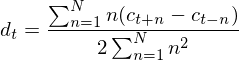
where  is a delta coefficient, from frame  computed in terms of the static coefficients  to . A typical value for  is 2. Delta-Delta (Acceleration) coefficients are calculated in the same way, but they are calculated from the deltas, not the static coefficients.

References 

Davis, S. Mermelstein, P. (1980) Comparison of Parametric Representations for Monosyllabic Word Recognition in Continuously Spoken Sentences. In IEEE Transactions on Acoustics, Speech, and Signal Processing, Vol. 28 No. 4, pp. 357-366

X. Huang, A. Acero, and H. Hon. Spoken Language Processing: A guide to theory, algorithm, and system development. Prentice Hall, 2001.

Matlab코딩한것을 해석하면서 진행합니다.

해밍윈도우 등은 Matlab함수로 구현 가능하지만 Java에서의 구현을 위하여 일일이 구현하였습니다.

사용한 음성은 umbrella.wav파일입니다.

%test STFT

clear

[Y,FS,NBITS, Readinfo]=wavread('umbrella.wav');

%umbrella.wav라는 파일을 볼러왔습니다. 

%Y      : 신호정보

%FS    : Sampling Frequency 22050Hz

%NBITS: BPS(Bit Per Sample), 16bit

%Readinfo : 파일헤더 구조체. 각종 정보 포함

sound(Y,FS);                                           %사운드 출력                 

len=length(Y);                                          %음성신호 길이

time=len/FS;                                            %파일의 재생시간: 초당 22050의 신호를 캡처하기 때문에 신호 Y의 길이가 20160이라면 재생시간은 0.9몇초가 된다.

figure;

x=linspace(1,time,len);                              %그래프의 시간축 설정. 0~0.9몇초를 신호의 길이만큼 분할

plot(x,Y);                                                 %신호 그래프 출력

%start stft

y=Y(1:len,1);                                        %음성신호를 y로 옮겨놓았음

%% windowing

R =2^9;                                                % R: window len. Windowing할 때의 창의 길이

W =0.54-0.46*cos(2*pi*(1:R)/R); W=W';   % w :해밍윈도우. 공식 적용한 값

N = 2^(nextpow2(length(W)));%2^9;        % N: FFT resolution.주파수 분해능,주파수, 그래프의 날카로움

L = ceil(R*0.1);                                    % L: number of non-overlap samples

overlap = R-L;                                     % Overlap(겹침처리)이 클수록 분해능이 좋음(속이 비거나 차는것) 현재 4

%%Type1

c=1;

h=(1+(len-R))/(1+R/2);                        %must be integer. 낮을수록 시간축 고분해능. R의 크기에 따라 자동으로 정수값으로 잡도록 하였음

h=fix(h*3/3);                                       %FS/h= overlap

d = zeros((1+R/2),1+fix((len-R)/h));

for b = 0:h:(len-R)                               %(b+1:b+R)의 길이=윈도우의 길이

  u = W.*y((b+1):(b+R));

  t = fft(u);                                           %해밍윈도우에 신호값을 곱해준 후 fft를 통하여 주파수도메인으로 분석

  d(:,c) = t(1:(1+R/2))';                         %각 윈도우 영역마다의 값을 대입

  c = c+1;

end;

time=linspace(0,timeleng,size(d,2));     %시간벡터. 재생시간을 그래프 배열크기에 맞추어 분할해줍니다.

freq=linspace(0,FS/2,size(d,1));          %주파수벡터. 위와 같은맥락

[X,Y]=meshgrid(time,freq);                  %3차원 그래프를 출력하기 위하여 2차원 평면 X와 Y 2개를 만듭니다.

figure;

mesh(X,Y,abs(d));                            %spectrogram 출력

STFT Type1

%%Type2

%Matlab내 함수 이용

[S F T] = spectrogram(y,W,overlap,N,FS);

%S : signal

%F : 관측할 수 있는 주파수배열

%T : 관측할 수 있는 시간배열. Overlap에 의한 분해능에 의존

                            %R에도 의존(Window 크기)

                            %R>Overlap

Z=abs(S);

[mX,mY]=meshgrid(T,F);    %2차원 평면 mX, mY 생성

figure;

mesh(mX,mY,Z);

figure;

contour(mX,mY,Z);            %등고선 그래프 출력

STFT_Type2

Contour 그래프

현재 Type1과 Type2의 Spectrogram의 정확도? 가 다르다는걸 눈으로 보아도 알 수 있습니다... 물론 보는 각도 때문에 그렇게 보일수도 있습니다만.

Type1의 경우 overlap을 계산하면 약290이 나옵니다.

반면 Type2의 경우 overlap을 490으로 설정해놓았습니다.

Type1의 h에 대한 식 h=fix(h*3/3); 에서 다음과 같이 바꾸어 보겠습니다.

h=2^(nextpow2(h));    이때 오버랩은 344정도 나옵니다. 그리고 그래프는

왼쪽이 Type1이고 오른쪽이 아까와 같은 오버랩의 Type2입니다. 거의 똑같죠?

굳이 nextpow쓸 필요는 없구요. h값을 낮추어주면 오버랩이 오릅니다. 오버랩이 클수록 그래프가 좀더 빽빽해지고 속이 덜 비겠죠?

Matlab함수에서 인수로 주는 오버랩 값 등의 제한에 대해서는 직접 함수를 사용해서 확인해보기 바랍니다.

위의 N은 nfft라고 FFT resolution입니다. 이 값이 낮으면 그래프가 삐죽빼죽 날카록게 되요. 덜 연속적이라서 그런거죠.

R값은 window길이인데, 매트랩 함수에서는 이 값도 잘 생각해줘서 넣어줘야 합니다. 높을수록 많은 정보를 담을 수 있겠지만 지나치면 연상량이 너무 많아지겠죠?

STF

2차원의 파워스펙트로그램입니다. 이걸 직접 구현할 수 있으면 좋겠는데 아직 거기까지는 잘 안되네요.

이부분은 추후에 구현하기로 하고 오늘 STFT는 여기서 끝!

다음편은 Mel-Filter bank 적용입니다.

영어발음 Apple에 Preemphasis를 해봅시다.

문제점 : 방음공간에서 된 샘플데이터라서 Preemphasis의 중요도가 낮아집니다. 잔기침 등등이 섞여있다면 좋겠습니다만..

추. Preemphasis 및 잡음제거는 나중으로 돌립니다.

우선은 특징추출부터 먼저 하고(음원이 깨끗하기 때문에) 유사도평가 후 잡음제거 및 Preemphasis를 하도록 하겠습니다

Matlab을 이용한 구현 및 신뢰도 확부후 Java로 재구현

설계부분. 미완성